Mastering Gradient Descent: Math, Python, and the Magic Behind Machine Learning — Part 1

Photo by Jeswin Thomas on Unsplash

Creating a Python class that computes gradient values automatically, similar to PyTorch tensors, is an excellent way to solidify your understanding of gradient descent.

Hello, everyone, and welcome! I’m Suraj Singh Bisht.

The machine learning industry is evolving rapidly, with new discoveries making waves in the field every day. As an observer, I’ve decided to embark on a journey to learn the basics of machine learning to stay updated. Before we dive into this series of articles, I want to make it clear that I’m not a professional data scientist. Instead, think of me as a new student who has recently started exploring this topic.

So, if you happen to come across any mistakes in my journey, please don’t hesitate to correct me.

You can connect with me here: https://www.linkedin.com/in/surajsinghbisht/

Introduction

In this article, I’ll explain what gradient descent is, why it’s crucial to learn, the basic math behind it, and how it benefits machine learning, and I’ll even provide a straightforward Python code example. This code example will simulate a PyTorch tensor class wrapper to automatically calculate gradient values, among other things.

I’m assuming you have a basic understanding of Python, some familiarity with fundamental math concepts, and a strong interest in delving into machine learning. If that describes you, then let’s proceed!

What is Gradient Descent?

Gradient Descent serves as an optimization technique employed to pinpoint the lowest point, known as a local minimum, in a function that can be differentiated. In the realm of machine learning, Gradient Descent is utilized to ascertain the values of a function’s parameters, such as coefficients. This process is executed in a manner that minimizes a cost function to the greatest possible extent.

In gradient descent, the gradient value, also known as the slope or derivative, measures how steep a function is at a particular point. It indicates the rate of change of the function with respect to its input variable.

In simple terms, think of the gradient value as a measure of how sensitive or influential an input value is on the output value after it undergoes mathematical processing within a function. It also indicates whether this influence is in a positive or negative direction. Using this gradient value we can easily calculate how much change to the input value can change output and in which direction.

Positive Derivative (dy/dx > 0):

• When the derivative of a function is positive at a particular point, it means that the function is increasing at that point.
• In terms of the graph of the function, if you draw a tangent line at that point, it will have a positive slope, indicating that as you move to the right along the curve, the function values are increasing.
• Think of it as moving uphill on a hillside. As you walk to the right (in the direction of increasing x), you are going uphill, and the slope of the ground is positive

Negative Derivative (dy/dx < 0):

• When the derivative of a function is negative at a particular point, it means that the function is decreasing at that point.
• In terms of the graph, if you draw a tangent line, it will have a negative slope, indicating that as you move to the right along the curve, the function values are decreasing.
• Think of it as moving downhill on a hillside. As you walk to the right (in the direction of increasing x), you are going downhill, and the slope of the ground is negative.

Zero Derivative (dy/dx = 0):

• When the derivative of a function is zero at a particular point, it means that the function has a flat spot or a local extremum (either a maximum or a minimum) at that point.
• In terms of the graph, if you draw a tangent line, it will be horizontal (with a slope of zero), indicating that the function is not changing at that point.
• Think of it as standing on a flat plateau. If you move to the right or left, the slope of the ground is flat, so you’re not going up or down.

For instance, suppose we have a function f(x) that takes a single input and, after applying some mathematical operations, produces a single output. Calculating the gradient value of this function entails assessing how even a slight change in the input value impacts the resulting output value of the function.

Let's see this in a graph

import matplotlib.pyplot as plt
import numpy as np

# simple function
def func(x):
    return np.sin(x)

# derivate of func(x)
def d_func(x):
    return np.cos(x)

X = np.arange(-5, 5, 0.4) # sample x values
Y = func(X) # y values
Z = d_func(X) # derivates/gradient value

plt.plot(X, Y, c="blue", marker='o', label="(X, func(X))")
plt.plot(X, Z, c='red', marker='o', label="(X, d_func(X))")
plt.xlabel('X')
plt.ylabel('Y/Z')
plt.legend()
plt.grid(True)
print("(X, func(X)) = ", list(zip(X[:2], Y[:2])))
print("(X, d_func(X)) = ", list(zip(X[:2], Z[:2])))

In this visual representation, the red line represents the derivative output, while the blue line represents the actual output.

Jupyter notebook output

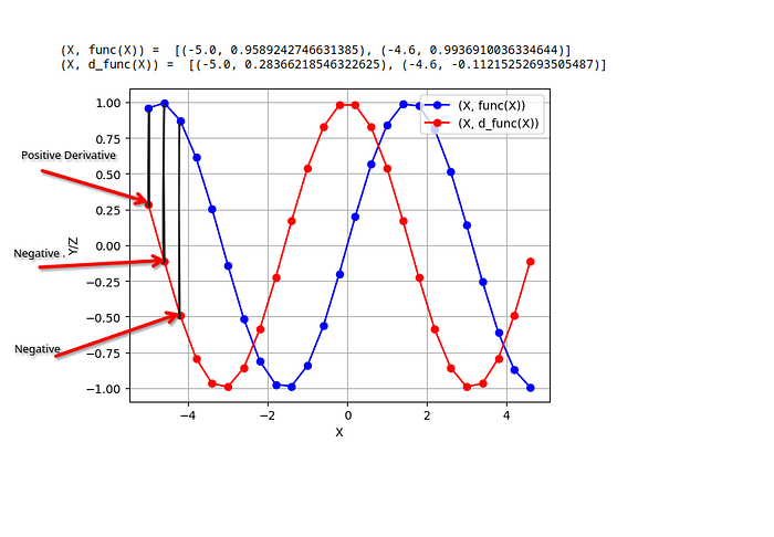
• Positive derivative: Function is increasing, slope is upward.
• Negative derivative: Function is decreasing, slope is downward.
• Zero derivative: Flat point, no change in slope (neutral).

This measurement of impact or sensitivity, which quantifies the relationship between the input and output values, is expressed as a numerical value referred to as the gradient value of that function.

More example,

1. f(x) = x, then the gradient value of this function is 1.
2. The gradient (or derivative) of the function f(x) = 2x is 2.
3. The gradient (or derivative) of the function f(x) = x² is 2x.

Let’s cross-verify the gradient values for the previous examples using the concept of input variations. To do this, we’ll use a small value, h = 1, and a fixed input value, x = 2.

Example 1:

Original Function: f(x) = x

When we pass (2 + h) as the input value, we get f(2 + h) = 2 + h as the output. This means the input remains the same.

A gradient value of 1 signifies that a change in the input value has the same effect on the output, just like in this case where the output (2 + h) follows the input (h).

Example 2:

Original Function: f(x) = 2x

When we pass (2 + h) as the input value, we get f(2 + h) = 4 + 2h as the output.

A gradient value of 2 implies that a change in the input value results in an output change that is twice as large, as observed here where the output (4 + 2h) is two times the input change (2h).

Example 3:

Original Function: f(x) = x²

When we pass (2 + h) as the input value, we get f(2 + h) = 4 + h² + 4h as the output.

A gradient value of 2x means that the effect of a change in the input value depends on the value of x. In this case, if x = 2 + h, then the output change (4 + h² + 4h) is influenced by 2 times the input change (2(2 + h))=4+2h, demonstrating how the gradient varies with the input value x.

The Basic Concept in Mathematics?

Derivative

A derivative measures how a function changes as its input (usually denoted as ‘x’) changes. In other words, it tells us the rate of change of a function at a specific point. You can think of it as the slope of a curve at a particular point.

To calculate a derivative, you can follow these steps:

1. Start with a function, let’s say f(x). For example, f(x) = 2x².
2. Choose a point at which you want to find the derivative. Let’s say x = 3.
3. Using the above equation to find the derivative at that point: f’(x) = lim (h -> 0) [f(x + h) — f(x)] / h
4. Here, ‘h’ is a very small number close to zero. It represents a tiny change in the x-value.
5. Plug in the values and calculate: f’(3) = lim (h -> 0) [2(3 + h)² — 2(3)²] / h
6. Calculate the limit as ‘h’ approaches zero to get the derivative at x = 3.

My Terminal (Python Output)

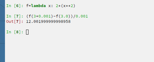
= 12

the derivative of f(x) = 2x² is f’(x) = 4x.

f’(3) = 4(3) = 12

Let’s see this in a graph

import matplotlib.pyplot as plt
import numpy as np

# simple function
def func(x):
    return 2*(x**2)

# derivate of func(x)
def d_func(x):
    h = 0.00001
    return (func(x+h)-func(x))/h

X = np.arange(-25, 25, 1) #
Y = func(X)
Z = d_func(X)

plt.plot(X, Y, c="blue",  label="(X, func(X))")
plt.plot(X, Z, c='red', label="(X, d_func(X))")
plt.xlabel('X')
plt.ylabel('Y')
plt.legend()
plt.grid(True)

Jupyter notebook Output

• Positive derivative: Function is increasing, slope is upward.
• Negative derivative: Function is decreasing, slope is downward.

How to find the derivative of a function?

The most fundamental way to find a derivative is by using the limit definition of a derivative. The derivative of a function f(x) at a point ‘a’ is defined as:

• f'(a) = lim (h -> 0) [(f(a + h) - f(a)) / h]

In this formula, ‘h’ is a small number that approaches zero. This limit expression calculates the slope of the tangent line as ‘h’ approaches zero.

Doing things this way can be very slow and uses up a lot of computer power. To make it easier, there are different shortcuts and tricks we can use. These tricks include the Power Rule, Sum/Difference Rule, Product Rule, Chain Rule, Trigonometric Functions, Exponential and Logarithmic Functions, and Quotient Rule.

If you want to learn more about these shortcuts in an easy-to-understand way, you can watch YouTube videos that explain them.

Gradient Descent

The mathematical concept behind Gradient Descent is rooted in calculus and the idea of finding the minimum (or sometimes maximum) of a function by iteratively adjusting the input parameters.

The algorithm iteratively adjusts the parameters (variables) of a model or function to minimize or maximize a specific objective (usually a cost or loss function). It does so by following the direction of the negative gradient (for minimization) or positive gradient (for maximization). When it encounters a point with a zero gradient, it may stop or change its behavior depending on the specific optimization algorithm being used.

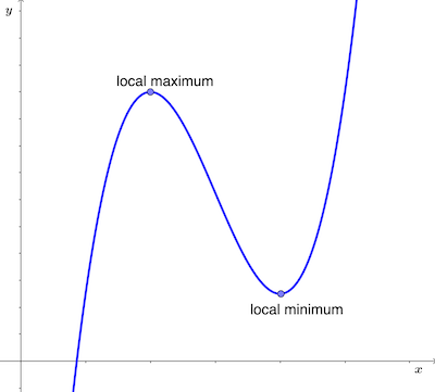
Local Minimum: A local minimum is a point on the function’s curve where the function has a lower value than its neighboring points but doesn’t necessarily have the lowest value in the entire function. In gradient descent, finding a local minimum is a key objective because it represents a potential optimal solution for the optimization problem. At a local minimum, the derivative (gradient) of the function is zero. This means that at that point, the function is flat, and moving in any direction would lead to an increase in the function’s value.

Local Maximum: A local maximum is a point on the function’s curve where the function has a higher value than its neighboring points but isn’t the highest value in the entire function. In some optimization problems, finding a local maximum might be the goal, though it’s less common than finding local minima. At a local maximum, like at a local minimum, the derivative (gradient) of the function is zero. This indicates that at that point, the function is flat, and any movement would result in a decrease in the function’s value.

The gradient descent update equation is a formula used to adjust the parameters of a model in order to minimize or maximize an objective function. It’s a critical part of the iterative process of finding the optimal set of parameters.

https://en.wikipedia.org/wiki/Gradient_descent

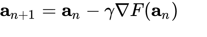
The equation above describes what the gradient descent algorithm does:

• aₙ₊₁ represents the value of the variable (parameter) at the next iteration.
• aₙ represents the current value of the variable (parameter) at the current iteration.
• α (alpha) is the learning rate, a small positive constant.
• ∇F(aₙ) represents the gradient of the function F with respect to the parameter aₙ.

To make it more simple to understand, we can write the above equation in this way.

New_Parameter = Old_Parameter — Learning_Rate * Gradient

• New_Parameter: This represents the updated value of the parameter you’re optimizing
• Old_Parameter: This is the current value of the parameter before the update.
• Learning_Rate: It’s a small positive number that determines the size of the step you take during each iteration.
• Gradient: The gradient is the derivative of the objective function with respect to the parameter you’re trying to update.

To understand the gradient descent update equation, it is important to understand what are cost estimation functions and how they are important in it.

No need to worry if things are still unclear. Before I provide more explanations, let’s make sure you understand what a cost estimation function, like Mean Squared Error, is.

Cost estimation function

A cost estimation function, such as Mean Squared Error (MSE), is a way to measure how well an algorithm is performing in solving a specific problem, typically in the context of machine learning or optimization.

In the case of MSE, it quantifies the average of the squared differences between the predicted values and the actual values in a dataset. A lower MSE indicates that the predictions are closer to the true values, while a higher MSE means that the predictions are further from the truth.

In simple terms, MSE helps you assess how accurate your model’s predictions are by measuring the error between what it predicts and what actually happens. The goal is to minimize this cost function to improve the model’s performance.

Example (Mean Squared Error):

Imagine you have a simple model that predicts the score a student is expected to get in a math test based on the number of hours they studied. You collect data for three students, and here are the actual scores and the predicted scores by your model:

Actual Scores: [80, 90, 70]

Predicted Scores: [75, 85, 75]

To calculate the MSE, you follow these steps:

1. Take the difference between the actual score and the predicted score for each student:

• For the first student: (80–75) = 5
• For the second student: (90–85) = 5
• For the third student: (70–75) = -5

2. Square each of these differences:

• (5)² = 25
• (5)² = 25
• (-5)² = 25

Calculate the average (mean) of these squared differences: (25 + 25 + 25) / 3 = 25

So, the Mean Squared Error (MSE) in this case is 25.

Joining all pieces

I assume that up to this point, you have a theoretical understanding of the concepts discussed. You’re familiar with what the gradient value represents, what a cost function is, and how to calculate the gradient of a function. Now, let’s connect these concepts to grasp how they come together to improve the accuracy of a machine learning model’s predictions. In simpler terms, we’ll explore how the process of utilizing a cost function, gradient descent, and parameter adjustments works to reduce errors in a prediction model and make it better at making accurate predictions.

Flow Of Model Training | Pardon my drawing skills :)

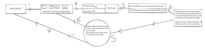
1. You start with a prediction model, which takes some input data and provides an output prediction. This model is controlled by certain parameters (often denoted as weights and biases). To measure how well your model is performing, you define a cost function (also known as a loss function or error function). This function quantifies the error between the model’s predictions and the actual target values. The cost function typically takes two inputs: the model’s predictions and the actual target values. It outputs a single number that represents the error. [Mean Squared Error (MSE)]
2. You use your model to make predictions on a set of training data.
   For each data point, you calculate the loss using the cost function by comparing the model’s prediction to the actual target value.
   The loss provides a measure of how far off the model’s predictions are from the truth for that particular data point.
3. Now, you want to minimize the overall loss across all the data points to improve your model. Gradient Descent comes into play here. Gradient Descent works by calculating the gradient (derivative) of the cost function with respect to the model’s parameters. This gradient points in the direction of the steepest increase in the cost function.
   To minimize the loss, you want to move in the opposite direction of the gradient, so you subtract the gradient from the current parameter values.
4. You update the model’s parameters using the gradient information obtained in the previous step. The update rule often involves a learning rate (α), which determines how big of a step you take in the direction opposite to the gradient. The formula for parameter updates typically looks like this: aₙ₊₁ = aₙ — α ⋅ ∇F(aₙ). check the above section.

As you iteratively update the parameters using Gradient Descent, the model learns to make better predictions that minimize the overall loss of the training data.

Understand By Example Codes.

To clarify the above-discussed topics, I’m providing a straightforward illustration of applying gradient descent to a linear regression problem.

In this example, we’ll start with a random set of input and output values. The output values will have some randomness associated with the input values. My aim is to show how gradient descent algorithms can be applied to adjust the slope and intercept of the linear regression line, minimizing the loss.

I’ll present this same example in three ways to demonstrate three different methods for calculating the gradient:

1. Finite Difference Approximation.
2. Derivative Equations.
3. Using an Automatic gradient value computing function.

Finite Difference Approximation.

This code demonstrates how gradient descent is used to adjust the parameters (weight and bias) of a linear regression model to fit noisy data. The goal is to minimize the mean squared error between the predicted and actual output values.

# approach using Finite Difference Approximation.
# Import necessary libraries
import matplotlib.pyplot as plt
import numpy as np

# an array ranging from -0.5 to 0.5 with a step of 0.01
inputX = np.arange(-0.5, 0.5, 0.01) 
# random values with a normal distribution to add noise to the input.
noise = np.random.normal(0, 0.2, inputX.shape)
# output values with noise.
outputY = inputX+noise
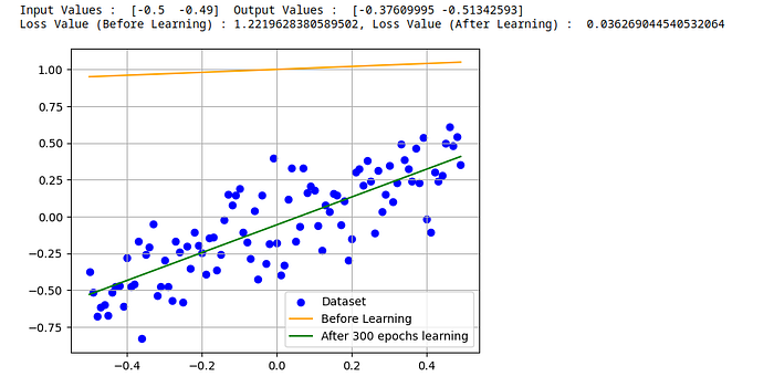
print("Input Values : ", inputX[:2], " Output Values : ", outputY[:2])
# so input dataset is ready inputX, outputY
plt.scatter(inputX, outputY, c="blue", label="Dataset")

# initial weights and bias
weight = 0.1 # any value
bias = 1 # any value

# calculates the predicted values based on the input, weight, and bias.
def linear_regression_equation(input_value, weight, bias):
    # X = independent value
    # Y = Dependent Value
    # M = SLOPE
    # B = INTERCEPT/BIAS
    # = y=mx+b
    predicted_value = (weight * input_value) + bias
    return predicted_value

# calculates the mean squared error (MSE)
def cost_function(input_value, weight, bias, target_value):
    predicted_value = linear_regression_equation(input_value, weight, bias)
    difference = (target_value - predicted_value)**2
    return sum(difference)/len(difference)

# calculates gradients using finite difference approximation.
def gradient_value_using_approx(inputX, outputY, weight, bias):
    # this approach is easy to implement but, 
    # it takes more computation power and time.
    f = cost_function
    h = 0.001
    w_grad_val = (f(inputX, weight+h, bias, outputY)-f(inputX, weight, bias, outputY))/h
    b_grad_val = (f(inputX, weight, bias+h, outputY)-f(inputX, weight, bias, outputY))/h
    return (w_grad_val, b_grad_val)

# the loss (MSE) before any learning
before_loss_value = cost_function(inputX, weight, bias, outputY)
plt.plot(inputX, linear_regression_equation(inputX, weight, bias), c="orange", label="Before Learning")

# training parameters
epochs = 300
learning_rate = 0.08
# Weights and bias are updated using the learning rate 
# and gradients to minimize the loss.
for _ in range(epochs):
    (w_grad_val, b_grad_val) = gradient_value_using_approx(inputX, outputY, weight, bias)
    weight = weight - (learning_rate*w_grad_val)
    bias = bias - (learning_rate*b_grad_val)

# the loss (MSE) after the specified number of epochs.
after_loss_value = cost_function(inputX, weight, bias, outputY)
print(f"Loss Value (Before Learning) : {before_loss_value}, Loss Value (After Learning) :  {after_loss_value}")
# plot the linear regression line in green
plt.plot(inputX, linear_regression_equation(inputX, weight, bias), c="green", label=f"After {epochs} epochs learning")
plt.legend()
plt.grid(True)

Output :

Jupyter notebook output

Derivative Equations.

The same code, but this time with Derivative Equations Method

#.... Same Code as given in previous example .... 
def gradient_value_using_rules(inputX, outputY, weight, bias):
    # recommended way
    # using chain rule to get derivate of 
    # cost_function(linear_regression_equation(input))
    #
    w_grad_val = sum((-2 *inputX)*(outputY - ((weight*inputX)+bias)))/len(inputX)
    b_grad_val = sum(-2*(outputY - ((weight*inputX)+bias)))/len(inputX)
    return (w_grad_val, b_grad_val)

#.... Just replace gradient_value_using_approx to gradient_value_using_rules ....

Same Result :

Machine learning models often involve complex architectures with layers, activations, and loss functions. For example, in a neural network, you have multiple layers with various activation functions. Calculating gradients manually for such models can be daunting, so to mitigate this issue we can use programming libraries like TensorFlow and PyTorch to automate this process, making it faster and less error-prone.

These libraries not only compute gradients but also provide a way to debug and inspect intermediate values during the backward pass. This is incredibly useful when diagnosing issues or implementing custom loss functions.

For this tutorial, instead of using PyTorch or TensorFlow, I’ve created a simple Python class wrapper to manage this task. By wrapping our parameters with this class object, we can easily calculate gradient values without any complex modifications. This class, behind the scenes, handles all the complexity and provides us with a user-friendly object. We can perform arithmetic operations on this object as usual, but in the background, it keeps a record of calculations and arithmetic operations. In the end, with a simple .backward method call, we can easily obtain the parameter's gradient value.

Automatic compute gradient value

Python class, which can compute the gradient value of parameters automatically.

class TensorValue:
    def __init__(self, num, ops= None, left=None, right=None):
        self.num = num
        self.ops = ops
        self.left = left
        self.right = right
        self.grad = 0.0
        self.leaf = True
        
        if self.left or self.right:
            self.leaf = False
    
    def __add__(self, y):
        return self.__class__(self.num + getattr(y, "num", y), ops="+", left=self, right=y)
    
    def __radd__(self,  y):
        return self.__add__(y)
    
    def __sub__(self, y):   
        return self.__add__(-y)
    
    def __rsub__(self,  y):
        return self.__add__(-y)
    
    def __mul__(self, y):     
        return self.__class__(self.num * getattr(y,"num", y), ops="*", left=self, right=y)
    
    def __rmul__(self,  y):
        return self.__mul__(y)
    
    def relu(self):
        return self.__class__(max(0, self.num), ops="rl", left=self)

    def __neg__(self):
        return self.__mul__(-1)
    
    def __truediv__(self, y):        
        return self.__mul__(y**-1)
    
    def __rtruediv__(self,  y):
        return self.__mul__(y**-1)
    
    def __pow__(self, y):
        return self.__class__(self.num ** getattr(y, "num", y), ops="pow", left=self, right=y)
    
    def __repr__(self):
        return f"{self.__class__.__name__}({self.num})<{id(self)}>"
    
    
    def flush_gradient(self):
        if not self.leaf:
            self.grad = 0
        if isinstance(self.left, self.__class__):
            self.left.flush_gradient() 
        if isinstance(self.right, self.__class__):
            self.right.flush_gradient()
    
    def backward(self):
        self.grad = 1
        return self.calculate_gradient_backward()
        
    def calculate_gradient_backward(self,):
        r = getattr(self.right, "num", self.right)
        l = getattr(self.left, "num", self.left)
    
        # the derivative of f(x, y) = x + y with respect to x is simply 1
        if self.ops=="+":
            self.left.grad += (self.grad * 1)
            if isinstance(self.right, self.__class__):
                self.right.grad += (self.grad * 1)
                
        # the derivative of f(a, b) = a * b with respect to 'a' is 'b'.
        elif self.ops=="*":
            self.left.grad += (r * self.grad)
                
            if isinstance(self.right, self.__class__):
                self.right.grad += (l * self.grad)
        
        elif self.ops=="rl":
            self.left.grad += (int(self.num > 0) * self.grad)
                
                
        # the derivative of f(a, b) = a^b with respect to 'a' is 'b * a^(b-1)'
        elif self.ops=="pow":
            self.left.grad += ((r * (l ** (r - 1))) * self.grad)
                
            if isinstance(self.right, self.__class__):
                self.right.grad += ((l * (r ** (l -1))) * self.grad)
        
    
        if isinstance(self.left, self.__class__):
            self.left.calculate_gradient_backward()
            self.left.flush_gradient()
            
        if isinstance(self.right, self.__class__):
            self.right.calculate_gradient_backward()
            self.right.flush_gradient()

Idea

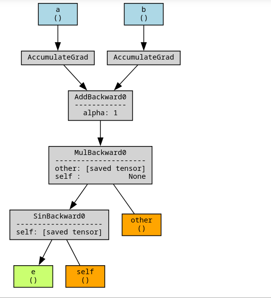
The central idea behind the TensorValue class is to maintain a computational graph in which each node represents a numerical value along with its gradient. This graph captures the sequence of mathematical operations performed on these values. When you perform operations using instances of TensorValue, new nodes are created in the graph to represent the results of these operations. The gradient information is tracked throughout this graph.

# Example : arithmetic operations between a & b PyTorch Tensor
c = (a + b)*2;
d = a * b
e = torch.sin(c)

# Visualizing the computation graph
make_dot(e, params={“a”: a, “b”: b})

Computation graph :

Jupyter notebook output

Explanation

This code defines a Python class called TensorValue that represents a numeric value with some additional functionality for gradient calculations.

• The class is initialized with a numeric value (num), optional operations (ops), and optional left and right operands (left and right). It also has attributes for gradient (grad) and whether it's a leaf node (leaf).
• The class overrides several arithmetic operators (__add__, __radd__, __sub__, __rsub__, __mul__, __rmul__, __truediv__, __rtruediv__, __pow__, __neg__) to allow operations on instances of TensorValue.
• The flush_gradient method resets the gradient values and the backward the method initiates the backward propagation for gradient calculation.
• The calculate_gradient_backward method calculates gradients based on the operation performed (addition, multiplication, ReLU, or exponentiation) and recursively propagates them to the operands.

Let’s use this class wrapper in the same example.

import matplotlib.pyplot as plt
import random

inputX = [i*0.01 for i in range(-50, 50, 1)] #
noise = [random.randrange(1, 100)*0.01 for _ in inputX]
outputY = [(x+y) for x,y, in zip(inputX, noise)]
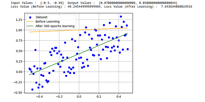
print("Input Values : ", inputX[:2], " Output Values : ", outputY[:2])

plt.scatter(inputX, outputY, c="blue", label="Dataset")


weight = 0.1 # any value
bias = 1.0 # any value
def linear_regression_equation(input_value, weight, bias):
    # X = independent value
    # Y = Dependent Value
    # M = SLOPE
    # B = INTERCEPT/BIAS
    # = y=mx+b
    predicted_value = (weight * input_value) + bias
    return predicted_value

def cost_function(input_value, weight, bias, target_value):
    c = 0
    for i,t in zip(input_value, target_value):
        predicted_value = linear_regression_equation(i, weight, bias)
        difference = (t - predicted_value)**2
        c += difference
    return c


def gradient_value_using_autograd_cal_wrapper(inputX, outputY, weight, bias):
    w = TensorValue(weight) # Here we are wrapping weight and bias
    b = TensorValue(bias)
    n = len(inputX)
    for x,y in zip(inputX, outputY):
        predicted_value = (w * x) + b
        loss = (y - predicted_value)**2
        loss.backward()
    return ((w.grad/n), (b.grad/n)) # Boom! simple



before_loss_value = cost_function(inputX, weight, bias, outputY)
plt.plot(inputX, [linear_regression_equation(i, weight, bias) for i in inputX], c="orange", label="Before Learning")
epochs = 300
learning_rate = 0.08
for _ in range(epochs):
    (w_grad_val, b_grad_val) = gradient_value_using_autograd_cal_wrapper(inputX, outputY, weight, bias)
    weight = weight - (learning_rate*w_grad_val)
    bias = bias - (learning_rate*b_grad_val)

after_loss_value = cost_function(inputX, weight, bias, outputY)
print(f"Loss Value (Before Learning) : {before_loss_value}, Loss Value (After Learning) :  {after_loss_value}")
plt.plot(inputX, [linear_regression_equation(i, weight, bias) for i in inputX], c="green", label=f"After {epochs} epochs learning")
plt.legend()
plt.grid(True)

Same Result :

Conclusion

In this article, we have explored the concept of gradient descent through various examples. We’ve covered the fundamentals of derivatives and differential equations, demonstrated how to compute the derivative of a function, discussed cost functions, introduced key concepts for refining linear regression parameters, and concluded with an example of an auto-gradient calculation class capable of automatically computing gradient values.

We’ve reached the end of this article. I hope you’ve learned something from this article. If you have, please share your thoughts and feedback in the comments section.

If you have any questions, you can ask in the comments or connect with me on LinkedIn.

Keep an eye out for the next part!